5 minutes
Graph Topology and Battle Royale Mechanics
The other day I found Alan Pike’s blog post from a few years ago which describes his iterative process for determining the order cities should be closed in the game Two Spies. Ultimately, finding a formal solution to city closing wasn’t necessary for the game, but it’s worth giving it a shot anyways since pruning by hand isn’t always convenient.
Closing cities is an important mechanic in the game, because as a sort of “battle royale” mechanic it prevents players from hiding in the corner of the map indefinitely. We can model the map as an undirected graph, where cities are vertices and travel routes are edges. Removing a city means deleting a vertex and its corresponding edges.
Closing cities without considering the resulting map can be suboptimal or unplayable. His post named two specific issues: disconnected graphs and path graphs (i.e. long lines of cities). A disconnected graph can result in a situation where the players can no longer interact. A path graph results in a map which isn’t very fun since the single path severely limits the strategies players can use.
The difficulty is that removing a city permanently changes the topology of the map. A choice might seem reasonable at one point but causes issues down the line. So picking the correct sequence of removals is important in maintaining a playable map.
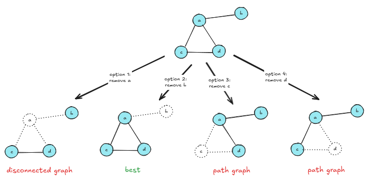
With the four nodes a, b, c, and d, there are four pruning options. However, option 1 results in a disconnected graph, and options 3 and 4 result in suboptional path graphs. Option 2 is the only one which maintains a connected, non-path graph.
Avoiding disconnected graphs
This one is simple enough. We just need to pick a city and perform a breadth-first search to ensure that every other remaining city is reachable from it. Since the map starts as a connected graph, we can always find a city to remove where the remaining graph is connected. This is because we can always find a node which isn’t an articulation point.
Avoiding path graphs
This one is fuzzier because intuitively this seems to be the case of better and worse graphs, rather than the previous case. So if we can come up with some metric for “better”, we can search for the “best” option and select it.
Intuitively, the reason that path graphs aren’t great is because as a hidden information game, the strategy of Two Spies relies on the fact that the opponent could be in multiple places at once, but path graphs reduce strategic possibility space and hidden state uncertainty.
We can quantify this by counting the number of steps it takes for every node to reach every other node. (For simplicity, we don’t have to count reverse paths. We don’t need to count A -> B and B -> A separately.) It turns out this measurement is called the Wiener number, the sum of the shortest paths between all nodes. Graphs with lower Wiener numbers are more optimal for the purposes of this game.
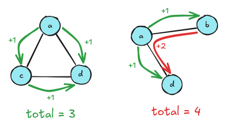
The graph on the left has a total distance of three, while the graph on the right (a path graph) has a total distance of four.
Greedy pruning
Since removing different cities results in maps with different Wiener numbers, it makes sense to 1) reject prunings that would result in disconnected graphs, and 2) select the pruning with the lowest Wiener number.
Unfortunately, this approach results in suboptimal graphs later on: the search process is discovering local minima rather than global minima. We can see on a large map of European cities (larger than used in the game) that although the pruning seems reasonable at first, we end up with a ring of cities at the end that can’t be pruned without resulting in a path graph. Not ideal.
Beam search
Rather than greedily removing the city which results in a graph with the lowest Wiener number, we should allow the pruning process to look ahead, rejecting prunings which inevitably result in bad final graphs. While an exhaustive search of the pruning combinations could be computationally infeasble for large graphs, that is likely not necessary.
To do this, we can borrow the idea of Beam Search, a classic AI search technique used heavily in natural language processing. Rather than greedily selecting one token at a time, we consider several options at the same time. In this case, rather than selecting tokens to decode, we are selecting cities to remove, and the beam is the sequence of cities which are removed. We score beams based on the average Wiener number of each of the graphs in the beam. This penalizes graphs which start with lower Wiener numbers but end with higher numbers than the alternative pruning sequences.
And as it turns out, pruning beams containing disconnected graphs and using a beam width of 10 works pretty well! We can see that the search algorithm avoided the trap of removing cities which would have resulted in a cycle, and instead prunes to a final, optimal triangle.
At the beginning of the pruning process, greedy and beam search behave almost identically. Both reduce the Wiener number smoothly as high-degree cities are removed around the edges.
The difference begins to appear when around half of the cities have been removed. Greedy pruning begins making locally optimal choices that restrict future structure. Beam search, by choosing the best removal sequences, avoids those locally optimal traps. Beam search ultimately results in a denser core.
The green line below shows the advantage of beam search over greedy at each step (i.e. Δ Wiener number). The moments where greedy pruning has an an advantage are the direct result of beam search optimizing long-term cumulative advantage.
The lesson here is that aesthetic contraints can sometimes be tackled using math, and sometimes “old school” techniques like Beam Search can come in handy in unexpected places, even outside of NLP contexts.